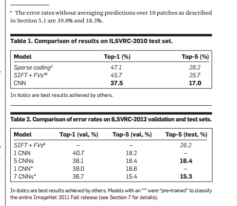
Abstract
We trained a neural network on the LSVRC-2010 dataset, which contains 1.2 million high-resolution images across 1000 categories. Our model achieved a top-1 error rate of 37.5% and a top-5 error rate of 17.0% on the test set. The architecture consists of 60 million parameters, 650,000 neurons, including 5 convolutional layers and 3 fully connected layers. To prevent overfitting, we implemented the Dropout technique. Additionally, we used this model in the ILSVRC-2012 competition, where it outperformed the second-place entry by achieving a top-5 error rate of 15.3%, compared to 26.2%.
1. Prologue
In the early days of neural networks, Yann LeCun and his colleagues faced rejection at major conferences when researchers believed that manual feature engineering was still necessary. In the 1980s, neuroscientists and physicists thought hierarchical feature detectors could be more robust, but they weren't sure what features these structures would learn. Some researchers discovered that multi-layer feature detectors could be effectively trained using backpropagation. The performance of the classifier for each image depended on the weights between connections.
Although backpropagation solved the training problem, it didn't meet expectations at the time, especially with deep networks, which often failed to produce good results. This led to frustration, but two years later, we realized the issue wasn't with the algorithm itself, but rather with the lack of sufficient data and computational power.
2. Introduction
This paper presents several key contributions:
1. We trained a convolutional neural network on ImageNet and achieved state-of-the-art accuracy.
2. We developed a GPU-accelerated implementation based on 2D convolutions and made it publicly available.
3. We introduced ReLU activation, multi-GPU training, and local response normalization to improve performance and reduce training time.
4. We used Dropout and data augmentation techniques to prevent overfitting.
5. Our architecture includes 5 convolutional layers and 3 fully connected layers, and reducing the depth significantly degraded performance.
(Due to hardware limitations, we used five 3GB GTX580 GPUs and trained the model for about 5–6 days.)
3. The Dataset
ImageNet is a large-scale dataset containing over 15 million images labeled into 22,000 categories, primarily sourced from the internet and manually tagged. The ILSVRC competition uses a subset of this dataset, consisting of around 1,000 categories, with approximately 1,000 images per class—totaling 1.2 million training images, 50,000 validation images, and 150,000 test images.
The ILSVRC-2010 dataset is the only version with labeled test sets, so we mainly used it for our experiments. However, we also participated in the ILSVRC-2012 competition. ImageNet only provides top-1 and top-5 error rates. Top-5 means the correct label is not among the top five predicted labels. Since ImageNet contains images of various resolutions, we resized all images to 256x256. For rectangular images, we first rescaled the shorter side to 256 and then cropped a central 256x256 region. We did not perform any other preprocessing except subtracting the mean pixel value.
4. The Architecture
The network has eight layers in total, with five convolutional layers and three fully connected layers. Below are some unique and important features of our design. We explain them in order of importance.
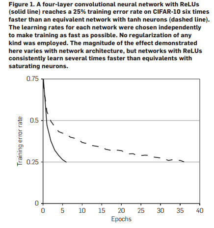
4.1. Rectified Linear Unit (ReLU) Nonlinearity
On a simple four-layer convolutional network, ReLU trains six times faster than the tanh function. Therefore, we used ReLUs to accelerate training and reduce overfitting.
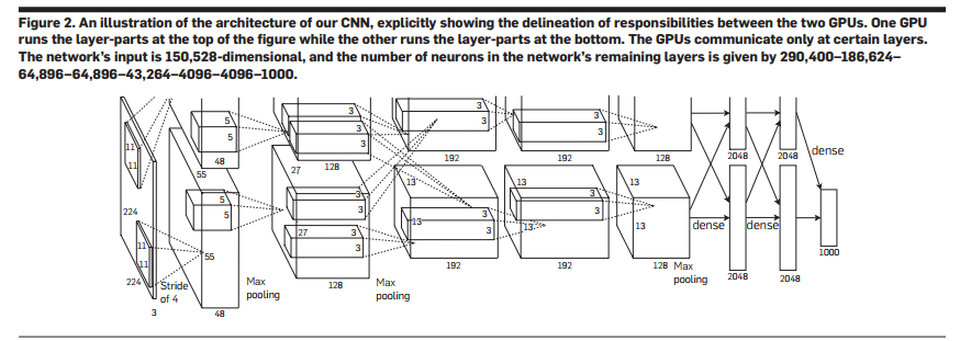
4.2. Training on Multiple GPUs
A single GTX580 GPU has only 3GB of memory, which limits the size of the network we can train. Experiments showed that 1.2 million training samples were sufficient, but too large for one GPU. So, we used two parallel GPUs, splitting the parameters and allowing communication only at certain layers. For example, the input to the third convolutional layer came from the entire second layer, while the fourth layer only received input from the same GPU’s third layer. Compared to training on a single GPU, this reduced the top-1 and top-5 errors by 1.7% and 1.2%, respectively, and slightly improved training speed.
4.3. Local Response Normalization
Although ReLUs don’t require input normalization to avoid saturation, they work well when inputs are positive. However, we found that adding local response normalization helped improve generalization.
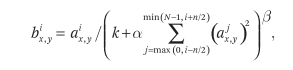
Using the formula above, we adjusted the relevant parameters during validation. We used k = 2, n = 5, α = 10â»â´, and β = 0.75. We applied normalization to ReLUs at specific layers. Experiments showed this reduced top-1 and top-5 errors by 1.4% and 1.2%, respectively. It also reduced the error rate on Cifar10 from 13% to 11% in a simple four-layer convolutional network.
4.4. Overlapping Pooling
Overlapping pooling reduced the top-1 and top-5 errors by 0.4% and 0.2%, respectively, and slightly increased the risk of overfitting.
4.5. Overall Architecture
Due to dual GPU training, the second, fourth, and fifth convolutional layers were only connected within the same GPU. The third convolutional layer was fully connected to the second. We used LRN in the first and second convolutional layers and max pooling in layers 1, 2, and 5. ReLU was used in every convolutional and fully connected layer.
5. Reducing Overfitting
5.1. Data Augmentation
The first method involved randomly cropping 224x224 images from 256x256 images and using horizontally flipped samples for training. During testing, we cropped 224x224 images from the four corners and center, and flipped them horizontally, resulting in 10 images per original image. After feeding them into the network, we averaged the softmax outputs to get the final result.
The second method involved adjusting the RGB values of the images, which slightly reduced the top-1 accuracy by 1%.
5.2. Dropout
The dropout layer does not participate in forward or backward propagation, so the network structure changes with each sample. We used a 0.5 dropout probability in the first two fully connected layers, which required doubling the number of training iterations to achieve convergence.
6. Learning Details
We used stochastic gradient descent (SGD) for training, with a batch size of 128, momentum of 0.9, and weight decay of 0.0005. Adding a small weight decay value was crucial for training, as it not only acted as a regularizer but also helped reduce the training error rate.
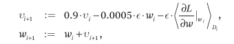
We initialized the weights with a Gaussian distribution (mean = 0, standard deviation = 0.01), and set the biases of the second, fourth, and fifth convolutional layers and the fully connected layers to 1. Other layers had biases set to 0. The learning rate started at 0.01 and was reduced by a factor of 10 three times (every 30 epochs), with a total of 90 epochs.
7. Results
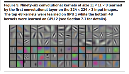
Interestingly, the two GPUs used for training focused on different aspects: one captured color information, while the other emphasized edge detection.
8. Discussion
It's worth noting that removing any of the convolutional layers significantly reduced the top-1 accuracy by about 2%, showing that the depth of the network plays a crucial role in our results.
Special Material Braided Sleeve
Special Material Braided Sleeve,Heat Proof Sleeve,Heat Proof Wire Sleeve,High Temperature Cable Sleeving
Shenzhen Huiyunhai Tech.Co., Ltd. , https://www.cablesleevefactory.com